ClusTree is
a self-extracting package. In order to install and
run the ClusTree tool,
please follow these three easy steps:
1. Download the
ClusTree.zip
file to your local drive.
2. Add the ClusTree
destination directory to your Matlab path.
3. In Matlab,type 'clustree' at the command prompt.
StartingClusTree
After typing 'clustree' at the command prompt the main window
will open.
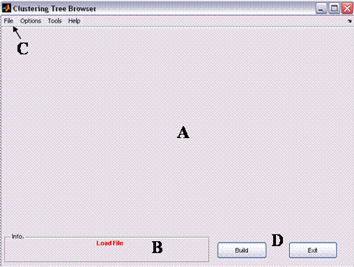
1. ClusTree: Main window
Figure 1: Clustree's main window
The main window consists of four areas:
A. Graphical window - Area
in which the graphical clustering result (i.e.,
the tree) is displayed. When no tree is loaded (e.g., prior the
clustering) this area will be empty.
B. Information area - the area in which the status is displayed (when
no data is loaded, a red ‘Load file’
indication is displayed). When a tree is loaded and
the external
classification is available (see Tree Options below) , three clustering
scores are displayed (see 1.2.i below).
C. Menus Bar - the area in which the some actions are available: data
loading, data processing, display options, detailed evaluation options
etc.
D. Command Buttons - 2 main buttons: ‘Build’ -
build a tree option (applicable only after clustering is applied) and
‘Exit’ - safely exiting the application.
Main
Workflow
1. New
clustering /Open ‘pre-clustered’ data
ClusTree can
either cluster a given dataset or analyze a
dataset that has already been clustered
i. New
clustering - analyzing a 'raw' dataset
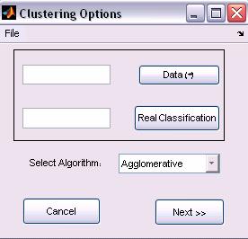
Figure 2: New Clustering options
ClusTree
receives three input
parameters, which are Matlab variables (i.e., must be defined in Matlab
workspace before
running the ClusTree).
Data (Mandatory field): two-dimensional matrix of doubles.
Represents
the elements (objects to be clustered are the matrix’s
columns).
Real classification (Optional
field): one-dimensional vector.
Represents the real classification of the elements (i.e., the class of
the i-th element which appears in the i-th place in the vector). Please note that
the vector’s length must be equal to the number of elements in
the Data matrix (Otherwise, an error will occurr and will be flagged).
The two input parameters can be typed in or
selected from the
base workspace.
Clustering Algorithms (Agglomerative, TDQC, PDDP)
Agglomerative Clustering: The Bottom-Up Agglomerative
clustering algorithm is the default option
of the Matlab environment (See Matlab, Statistics Toolbox 5.1 manual).
Please schoos the Data representation, Distance measure and
Linkage type options.
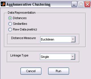
Figure 3:
Agglomerative Clustering options
a. Data Representation: the
input data matrix can be represented in various ways
Distances: a symmetric squared matrix in which the
value in the ij
place represents the distance between elements i and j.
Similarities: a
symmetric squared matrix in which the value in the ij place represents
the similarity between elements i and j.
Raw Data: a features-space matrix, which the value in
the ij place
represents the value of feature j for element i.
The user should specify in which of the
three options the data is
represented. If the data representation is either Distances or
Similarity, the Distance Measure option is disabled and ignored.
Otherwise (Raw data), the user should select one of the Distance
Measure options.
b. Distance Measure
euclidean
seuclidean
cityblock
mahalanobis
minkowski
cosine
correlation
hamming
jaccard
chebychev
c. Linkage Type -
After the distance is measure, a linkage is applied. The Linkage types
are:
single
complete
average
weighted
centroid
median
ward
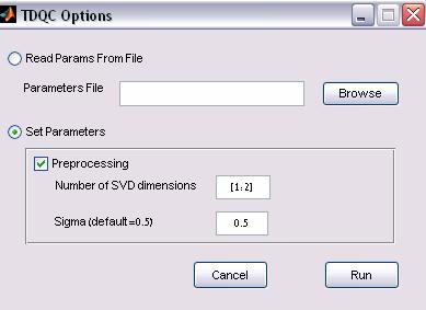
2. Top-Down-Quantum-Clustering
(TDQC) Options: the options can be specified in a
configuration file (advanced
mode), or by setting the parameters.
Figure 4: TDQC Clustering options
a. Parameter file option: The
TDQC can be applied to a configuration input file. The input file
format is as follows:
% A
line that starts with a ‘%’ is a
comment % data=[m*n
data matrix] * mandatory
data=x %realmapping=[1*n
classification] optional
realmapping=y %preprocessing=
[0-no, 1 - SVD, 2 - SVD + normalization]
preprocessing=2 % algorithm=4
--> must remain constant!
algorithm=4 %dims=[start:end]-->
dimensions
dims=[1:2] %clustercolumns=1
--> must remain constant!
clustercolumns=1 %steps=[for
gradient
descend]
steps=50 %numelems=[
number of elements]
numelems=200 %sigma=[for qc]
sigma=0.5
b. Direct input option
Preprocessing –
whether to cluster normalized, truncated SVD vectors (selected by
default)
Sigma value – the
Parzen window size (default is 0.5).
Once the algorithm is chosen and applied, the status message in the
information bar is changed to ‘loaded’
ii. Open
previously
saved results
Browsing previously saved file. The file is a Matlab data file
(.mat)
with two parameters: parent (required) and realClass (optional)
parent:
an (m-1)-by-3 matrix. The output of the Matlab
‘linkage’ function. parent is an containing cluster
tree information. The leaf nodes in the cluster hierarchy are the
objects in the original data set, numbered from 1 to m. They are the
singleton clusters from which all higher clusters are built. Each newly
formed cluster, corresponding to row i in parent, is assigned the index
m+i, where m is the total number of initial leaves. Columns 1 and 2,
parent (i,1:2), contain the indices of the objects that were linked in
pairs to form a new cluster. This new cluster is assigned the index
value m+i. There are m-1 higher clusters that correspond to the
interior nodes of the hierarchical cluster tree. Column 3, parent
(i,3), contains the corresponding linkage distances between the objects
paired in the clusters at each row i.
Note: ClusTree ignores the 3rd column (the linkage
distances).
realClass
(Optional field) - one-dimensional vector. Represents the
real classification of the elements (i.e., the class of the i-th
element appears in the i-th place in the vector). Please note that, the
vector’s length must be equal to the number of elements in
the Data matrix (Otherwise an error will occur).
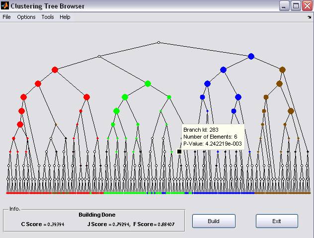
2. Build
the tree
the "Build tree" option is applicable after data is clustered or a
pre-clustered data is successfully loaded. Clicking the
‘Build’ button (area D) will construct the tree
The clustering tree represents a parent-child relation in
which the
leaf nodes represent data-elements and tree branched represent a
cluster (that includes the nodes below).
If the real classification information is available and paint level is
set to branches (see 3 below), clustering evaluation can be
presented. Since each node specifies a cluster, enrichment p-values can
be calculated to assign the given node with one of the classes in the
data. This is done by using the hypergeometric probability density
function. The significance p-value of observing k elements assigned by
the algorithm to a given category in a set of n elements is given by, where K is the
total number of elements assigned to the class (the
category) and N is the number of elements in the dataset. The p-values
for all nodes and all classes may be viewed as dependent set
estimations; hence we apply the False Discovery Rate (FDR) criterion to
them requiring q<0.05 [1]. P-values which do not pass this
criterion are considered non-significant. We further apply another
conservative criterion; namely, a node is considered significant only
if k≥n/2 (i.e., the majority of its elements belongs to the
enriched category).
In the graphical results, Dot sizes indicate statistical enrichment
levels (larger sizes correspond to smaller p-values). Uncolored nodes
represent non-significant enrichment (for modifications of the above
configurations see 3 below).
Branch information
By selecting a tree branch, a tooltip floating window appears
(Figure
5). The tooltip displays the Branch id, number of elements it includes,
and the significance enrichment p-values. The list of elements that
belong to the selected branch can be exported using the export command
(see ‘Export current’ below)
Scoring the Tree
1. C Score
– the relative number of significant branches (clusters)
[#significant branches/ the # of branches in the tree]
2. J Score We define
the weighted best-J-Score
,
where J*i
is the best J-Score
where tp is
the number of true positive cases, fn the number of false negative
cases and fp the number of false positive cases), for class i in the
tree, ni is the number of data-points (i.e., elements) in
class i, c is the number of
classes and N is the number of data-points in the dataset. This
criterion provides a single number specifying the quality of the tree
based on a few nodes that contain optimal clusters.
3. F Score
– similarly to the J Score, the weighted
best-F-Score
,
where F*i is the best
F-Score,
where ,
for class i in the tree, ni
is the number of data-points in class i, c is the number of classes and
N is the number of data-points in the dataset
3. Analyze
the tree
In addition to the visualization and scoring options, ClusTree
provides additional analysis tools (scores Distribution and
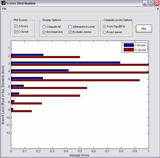
Ultrametric Display) i. Scores
Distribution
Figure 6: Visualization Scores Distribution
The Scores Distribution displays the Levels scores. A level l of the
tree contains all nodes that are separated by l edges from the root,
i.e., that share the same Breadth First Search (BFS) mapping. Each
level specifies a partition of the data into clusters. Choosing for
each node, the class for which it turned out to have a significant node
score, we evaluate its J-score (see above). If the node in question has
been judged to be non-significant by the enrichment criterion, its
J-score is set to null. The level score is defined as the average of
all J-scores at the given level.
In addition to the above definitions, the Levels C scores can be
displayed and some modifications can be applied (displaying the number
of branches in each level, including non-significant branches and
computing levels from leaf nodes instead of from the root, see Figure
6).
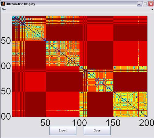
ii. Ultrametric
Display
The resulting tree defines
an Ultrametric dimension, where the distance
between two leaf-nodes is defined as the number of edges connecting
them.
The Ultrametric information is graphically displayed and can be
exported in a textual format
Figure 7: Ultrametric Display.
Additional
Functionalities
Export current branch: If a branch is selected (see Branch
information above and Figure 5),
its properties can be exported to either a set of Matlab variables or
to a text file.
Print graphical information
– printing the graphical results of the clustering (i.e., the
tree)
Save current
results – save the current environment for future analysis
(output file can be served as an input file, see ‘Open
previously saved results’ above)
4.
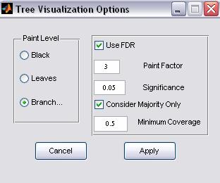
Visualization Options
Figure 8: Visualization options
ClusTree allows
the configuration of the default visualization settings.
Paint Level
Black –
regardless if the real classification is available or not, the tree is
displayed as black (i.e., nodes and branches are not colored). If this
option is selected all clustering evaluation information is not
available.
Leaves
(applicable only if real classification is available) - leaf nodes are
colored according to their classification association
Branches
(default) - (applicable only if real classification is available)
– both leaf nodes and branches are colored (for more
information, see 2 above).
FDR
(False Discovery Rate)
Option: The p-values for all nodes and all classes may be viewed as
dependent
set estimations; hence we suggest applying the False Discovery Rate
(FDR) criterion to them. Nevertheless, if user prefers not to apply FDR
correction, the FDR option should be unselected.
Paint Factor:
the number indicates the relative size of the nodes size.
Note: This option is for visualization purposes only.
Significance:
the p-value threshold for specifying a significant branch
Majority
Consideration: if this option is checked, the user can
specify a coverage threshold
for coloring a branch (values range from 0 to 1). For example if the
user specifies 0.5, A branch is considered significant only more than
50% of its elements belong to the enriched cluster. Please note: the value 1
means a ‘complete homogeneity’ (i.e., all the
elements in every colored branch belong to the enriched cluster)
Optional extensions
ClusTree is a set of self explanatory and documented Matlab
functions
and as such can be extended. Users who are familiar with Matlab and
wish to change features in the current tool are welcome to do so. In
addition, the tool was designed so that adding a new clustering method requires changing only one function.
Requirements
1. Project
name: ClusTree: The Hierarchical Clustering Analyzer
2. Project
home page: http://adios.cs.tau.ac.il/clustree/,
http://www.protonet.cs.huji.ac.il/clustree
(alternative)
3. Operating system(s): Platform independent tested on
MS-Windows (2000,
XP), Linux and Unix
4. Programming language: Matlab
5. Other requirements: Matlab 7 or higher,
Statistics Toolbox 5.1, COMPACT, and the PDDP package (optionally,
should be downloaded separately from
http://www-users.cs.umn.edu/~boley/PDDP.html)
6. License: Matlab
7. Any restrictions
to use by non-academics: open for all academic users.
Adequate referencing required. Non-academic users are required to apply
for permission to use this product.
References
[1] Benjamini, Y. and Hochberg,
Y. Controlling the False Discovery Rate: A Practical and Powerful
Approach to Multiple Testing. Journal of the Royal Statistical Society.
Series B (Methodological), 57 (1). 1995, 289-300.
 , where K is the
total number of elements assigned to the class (the
category) and N is the number of elements in the dataset. The p-values
for all nodes and all classes may be viewed as dependent set
estimations; hence we apply the False Discovery Rate (FDR) criterion to
them requiring q<0.05 [1]. P-values which do not pass this
criterion are considered non-significant. We further apply another
conservative criterion; namely, a node is considered significant only
if k≥n/2 (i.e., the majority of its elements belongs to the
enriched category).
, where K is the
total number of elements assigned to the class (the
category) and N is the number of elements in the dataset. The p-values
for all nodes and all classes may be viewed as dependent set
estimations; hence we apply the False Discovery Rate (FDR) criterion to
them requiring q<0.05 [1]. P-values which do not pass this
criterion are considered non-significant. We further apply another
conservative criterion; namely, a node is considered significant only
if k≥n/2 (i.e., the majority of its elements belongs to the
enriched category). ,
, 
 ,
,  where
where ,
,