Quantum clustering
Horn and Gottlieb have recently
suggested a clustering algorithm that can be applied reasonably efficiently to
a wide range of data types [9]. The Quantum Clustering (QC) algorithm[1], which is
briefly described here, begins with a Parzen window approach, assigning a
Gaussian of width σ to each data-point, thereby constructing ![]() , which can serve as a probability density that generates the
data. One then proceeds to construct a potential function
, which can serve as a probability density that generates the
data. One then proceeds to construct a potential function ![]() , where
, where![]() , thus rendering V positive definite. V develops minima that
are identified with cluster centers. Figure [11] presents an example for such a
potential function. The data come from the yeast data of Spellman [21],
presented in a compressed, normalized two-dimensional space [following a
preprocessing step]. The Z axis is the potential value V of each data-point
(using σ = ½). Spellman has identified 5 groups in the data (see the 5
different colors). In this case, four local minima are generated.
, thus rendering V positive definite. V develops minima that
are identified with cluster centers. Figure [11] presents an example for such a
potential function. The data come from the yeast data of Spellman [21],
presented in a compressed, normalized two-dimensional space [following a
preprocessing step]. The Z axis is the potential value V of each data-point
(using σ = ½). Spellman has identified 5 groups in the data (see the 5
different colors). In this case, four local minima are generated.
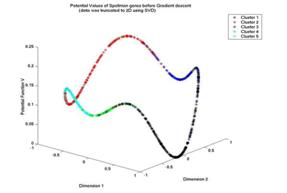
Fig. 1. The potential function V generated from a set of 798 data points using the parameter value σ = 1/2.
Once the minima of V(x) are defined as cluster centers, the assignment of data points to clusters can proceed through a gradient descent algorithm allowing auxiliary point variables yi(0) = xi to follow dynamics of yi(t+Δt) = yi(t) – η(t)ÑV(yi(t)) that lead to asymptotic fixed points yi(t) → zi coinciding with the cluster centers. Horn and Axel (2003), showed that the complex problem of finding those minima can be simplified to analysis of the data points only, thus reducing the time complexity to O(k∙N), where k is the number of dimensions after the SVD reduction and N is the number of data points (the potential at each point is a function of all other points. They also showed that gradient descent process involves calculation in the order of O(c*r*N2) where c is the number of iterations required for convergence (for most practical cases, 30-50 iterations were found to be sufficient).